Author: Ben Anderson (b.anderson@soton.ac.uk, @dataknut)

There is often talk in the media about the ‘spikes’ in energy demand caused by breaks in television schedules – when everyone is supposed to jump up and put the kettle on (or whatever). Although these make for good media stories, the largest overall surges are probably to do with cooking and secondary demands such as calls on industrial infrastructure while increasing ‘on demand’ and thus de-sychronised media consumption will mitigate the effects. That said, there doesn’t seem to be much evidence on what actually happens in households, partly because most measurement takes place at levels in the electricity grid where household and industrial demand cannot be separated. So we thought we’d take a look.

This analysis uses a stratified random sample of several thousand households from the County of Hampshire, the Isle of Wight and the Cities of Southampton and Portsmouth who are taking part in a large-scale study of energy demand. This sample is representative of these areas but possibly not of the wider UK population and we have been collecting 10 second power demand data from these households since late 2016.

Christmas Day 2016: Just another Sunday?

In order to compare household demand patterns for Christmas Day 2016 (a Sunday) with neighbouring Sundays we extracted and aggregated the 10 second power demand data to give mean kW demand over each 1 minute and 5 minute period for the Sundays before and after Christmas Day. This gives the plot shown below which also has 95% confidence intervals for the mean kW. These confidence intervals tell us several things, including how much variation there is at each time point.

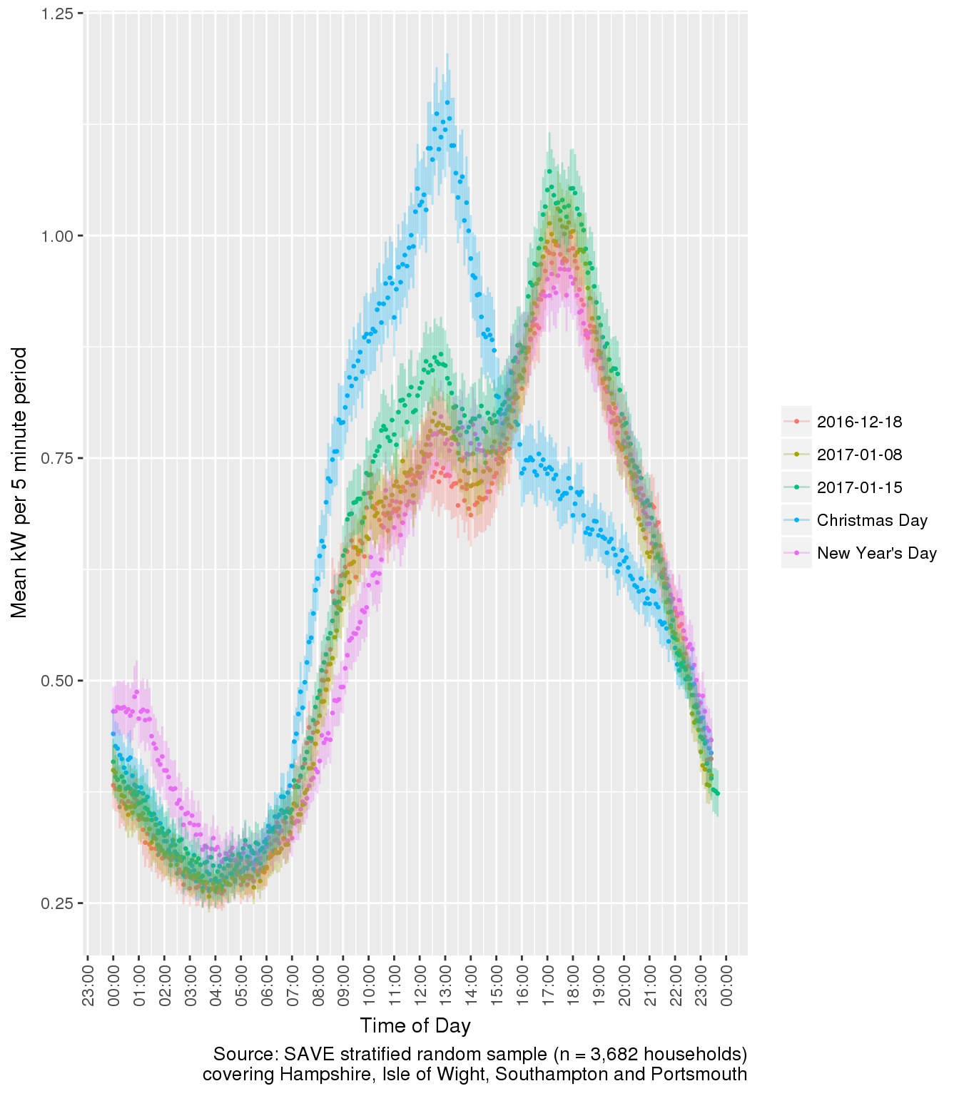
As we can see, Christmas Day is definitely not just another Sunday. Demand is slightly higher in the early hours of the morning than on other Sundays – perhaps Santa Claus is leaving the lights on? In contrast to other Sundays, demand trends steadily upwards earlier in the morning with the predicted ‘cooking‘ peak at around 13:00. It then falls away past the Queen’s Speech at 15:00 and on into a gentle evening at just the time that ‘normal’ Sundays are ramping up.

Interestingly New Year’s Day was almost just another Sunday but with some differences: demand from New Year’s Eve spilled over into the early hours and the usual breakfast surge was notably delayed by a couple of hours as we might expect.

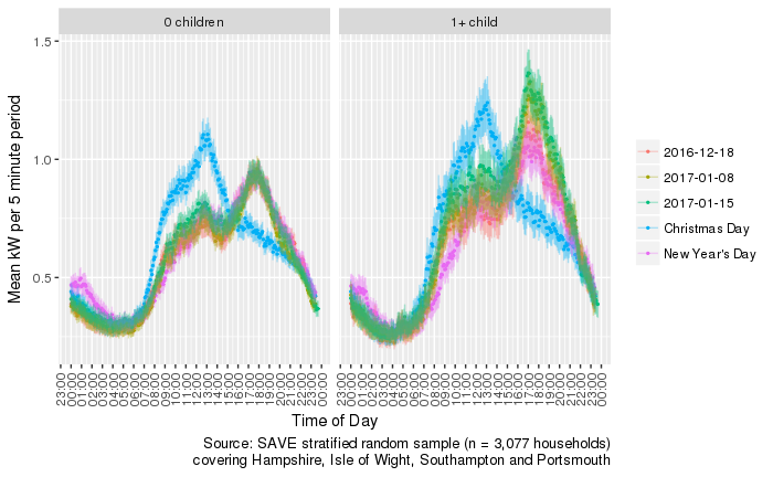
If we separate the plots out according to households with/without children we see more or less the same picture. However, households with children have higher power demand (although they are also likely to have more people in them) and this is especially true on ‘normal’ Sunday evenings. They appeared to go to bed slightly earlier on New Year’s Eve but get going rather later and have lower than normal demand on New Year’s Day evening compared to those without children. The latter appeared to party slightly later but be ‘back to normal’ by the evening – perhaps because many would have been at work on the Monday.

Can we spot the schedules?

So much for Sundays. Can we use the finer-grained 1 minute data to detect people’s behaviour? The plots below show the period 14:00 to 22:00 on Christmas Day with annotations.

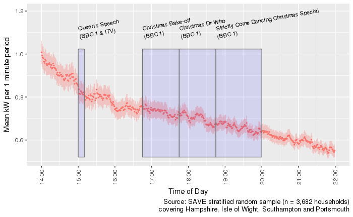
There is a visible dip in demand around 15:00 coinciding with the Queen’s Speech and this appears to be preceded by a slight plateau in the otherwise continuous decline in demand. Perhaps people were making drinks or otherwise ‘getting ready’ before Her Majesty spoke?

There is an unexplained visible dip at 16:00 followed by a possible spike at the end of the BBC’s Christmas Bake-off and an even smaller spike at the end of the BBC’s Strictly Come Dancing.

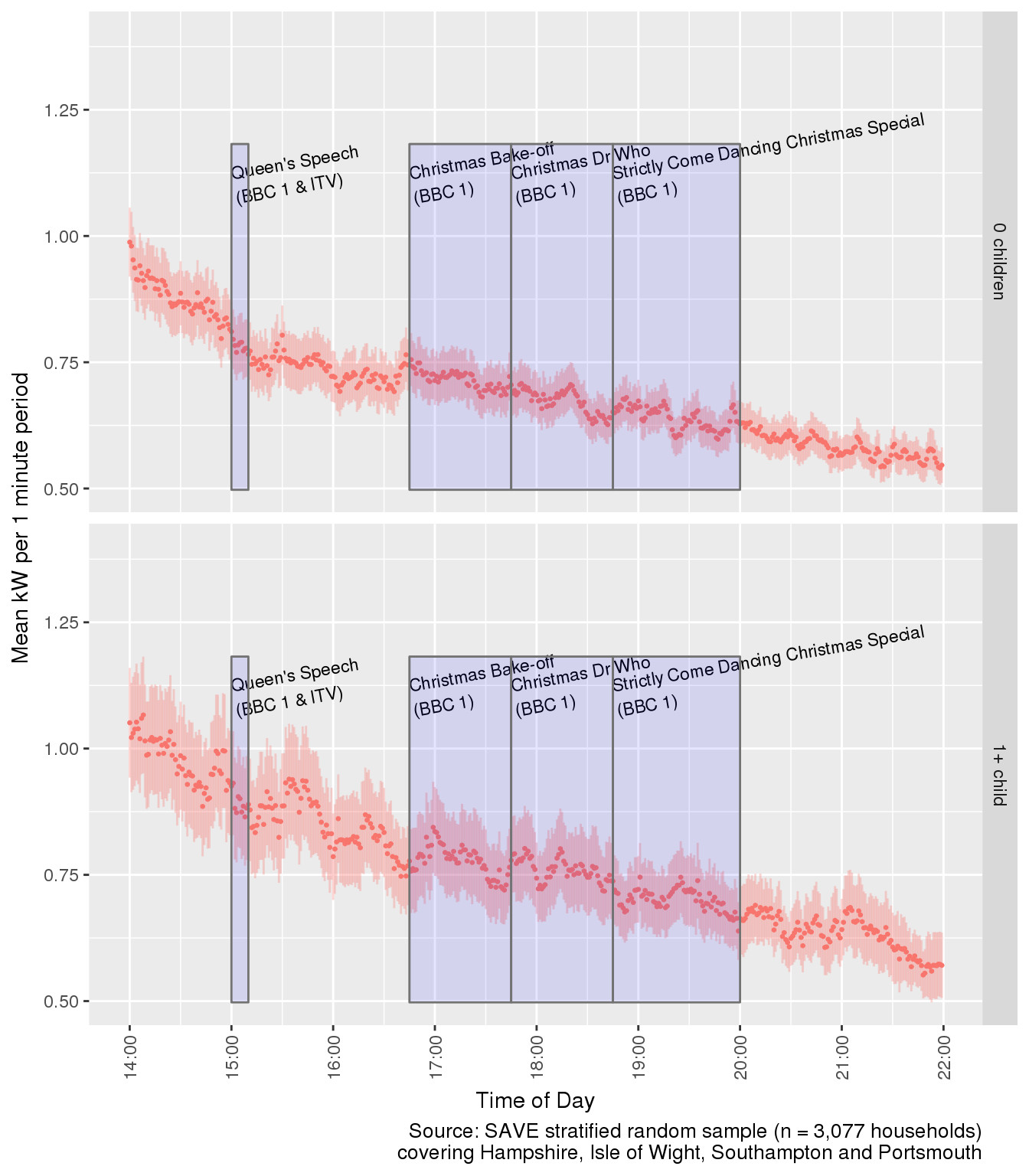
Separating out households with and without children (below) shows that the ‘plateau’ before 15:00 was mostly due to households with children as is the 16:00 dip and the post-Bake-Off spike. The post-‘Goodbye Len’ spike at 20:00 was, however much more likely to be households without children.

Finally, if we separate out household by the age of the Household Response Person (HRP – who completed the survey), we see that it is the ‘younger’ households who appear to reach for the appliances at the end of Dr Who and sometime after Strictly;  ‘middle-aged’ households who seemed to spike at the end of Strictly and ‘older’ households (HRP aged 55+) who pay most attention to Her Majesty…

About

The work was funded by the Low Carbon Network Fund (LCNF) through the Solent Achieving Value from Efficiency project. The analysis was generated using knitr in RStudio with R version 3.4.4 (2018-03-15) running on x86_64-redhat-linux-gnu. Analysis completed in 1056.318 seconds (17.61 minutes).

R packages used for base SAVE data processing:

• base R – for the basics (R Core Team 2016)
• data.table – for fast (big) data handling (Dowle et al. 2015)
• Hmisc – for capitalize (Harrell Jr, Charles Dupont, and others. 2016)
• lubridate – for fast date/time conversions (Grolemund and Wickham 2011)
• readxl – reading .xls(x) (Wickham and Bryan 2017)
• readr – fast .csv reading and parseing (Wickham, Hester, and Francois 2016)
• dplyr – data munching (Wickham and Francois 2016)
• dtplyr – data.table data munching (Wickham 2016)

Additional R packages used:

• ggplot2 – slick graphics (Wickham 2009)
• knitr – to generate reports (Xie 2016)

Data Access

Staff and students at the University of Southampton can apply to use anonymised versions of this data for research purposes.

References

Dowle, M, A Srinivasan, T Short, S Lianoglou with contributions from R Saporta, and E Antonyan. 2015. Data.table: Extension of Data.frame. https://CRAN.R-project.org/package=data.table.
Grolemund, Garrett, and Hadley Wickham. 2011. “Dates and Times Made Easy with lubridate.” Journal of Statistical Software 40 (3): 1–25. http://www.jstatsoft.org/v40/i03/.
Harrell Jr, Frank E, with contributions from Charles Dupont, and many others. 2016. Hmisc: Harrell Miscellaneous. https://CRAN.R-project.org/package=Hmisc.
R Core Team. 2016. R: A Language and Environment for Statistical Computing. Vienna, Austria: R Foundation for Statistical Computing. https://www.R-project.org/.
Wickham, Hadley. 2009. Ggplot2: Elegant Graphics for Data Analysis. Springer-Verlag New York. http://ggplot2.org.
———. 2016. Dtplyr: Data Table Back-End for ’Dplyr’. https://CRAN.R-project.org/package=dtplyr.
Wickham, Hadley, and Jennifer Bryan. 2017. Readxl: Read Excel Files. https://CRAN.R-project.org/package=readxl.
Wickham, Hadley, and Romain Francois. 2016. Dplyr: A Grammar of Data Manipulation. https://CRAN.R-project.org/package=dplyr.
Wickham, Hadley, Jim Hester, and Romain Francois. 2016. Readr: Read Tabular Data. https://CRAN.R-project.org/package=readr.
Xie, Yihui. 2016. Knitr: A General-Purpose Package for Dynamic Report Generation in R. https://CRAN.R-project.org/package=knitr.